Teaching with TwoRavens:
Replicating Fearon and Laitin (2003)

Fearon and Laitin (2003) is a landmark study on civil wars. It shows that many of the post-Cold War civil conflicts were not due to ethnic differences, but rather to factors that enabled insurgencies to thrive. These factors include mountainous terrain, low GDP, high population, and political instability.
 
This document will guide you through a replication of the statistical results in Fearon and Laitin (2003) using TwoRavens.

1 Access the data

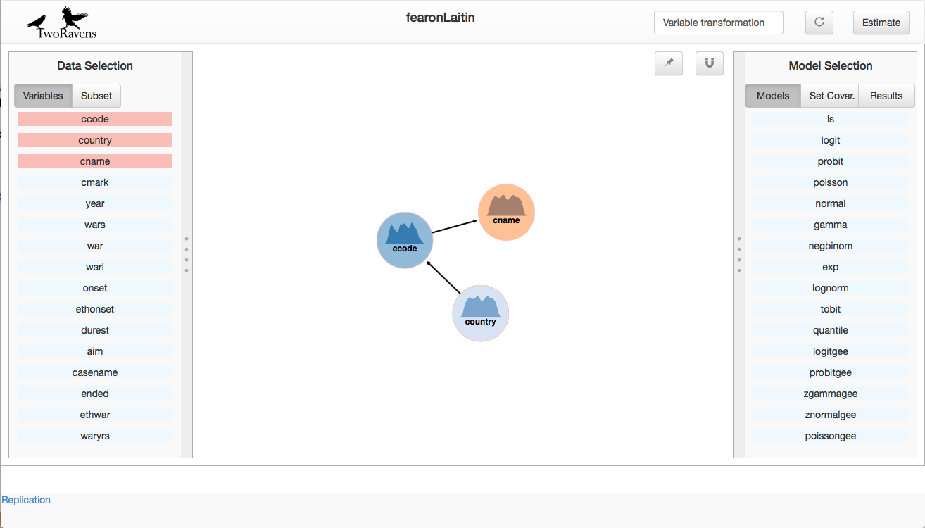
Follow the link to the Teaching with TwoRavens dataverse. Click on the Fearon and Laitin replication dataset. Next to the “Download” button for the file repdata2.tab, click “Explore.” This should open a page, as shown in figure 1.¹

In this module we will replicate the statistical analyses presented in Fearon and Laitin (2003). Their replication file, retrieved from http://web.stanford.edu/group/ethnic/publicdata/publicdata.html, reads as follows:

This is a replication script for Stata, so some knowledge of Stata syntax is required. logit means that we are using the logistic regression. The first variable name after logit is the dependent variable, which in this case is either onset, ethonset, emponset, or cowonset. In Stata syntax, the variable names following the dependent variable are the independent variables.

All of these variables are listed in the Data Selection panel of TwoRavens, under the Variables tab. If you mouseover these variable names, or click on them and mouseover the pebble in the center panel, you can view additional summary statistics, a brief description of the variable, and see its distribution.

Note that for Model #2, Fearon and Laitin subset the data for all observations where second > 0.49999, and estimates the model on that subset. Finally, the no log at the end of each line suppresses some of the information that Stata automatically prints to the console, and is not relevant for us here.

2 Instructions for Replicating Fearon and Laitin Models

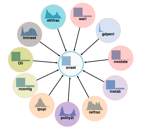
Begin with a clear modeling space. This means no variables are selected and thus no pebbles are in the center panel.

• Click the magnet button in the top right of the center panel
• Alternatively, click each selected variable name in the variable list in the left panel

2.1 Model #1

• Click the names of all the variables in Model #1 in the left panel
  • onset warl gdpenl lpopl lmtnest ncontig Oil nwstate instab polity2l ethfrac relfrac
• Mouseover onset and select Dep Var to tag onset as the dependent variable
  • The onset pebble should have a light blue outline and no fill color, signaling that this pebble has been tagged as the dependent variable
• Right click on each independent variable to create an arrow, and left click on onset to draw an arrow from the IV to the DV
  • These arrows signify the direction of the relationship

The resulting image in the center panel should appear like figure 2. Now that the relationships among variables have been specified, we now select the appropriate statistical model:

• Click on logit in the Model Selection panel on the right, under the Models tab

At this point, the variables have been selected, the relationships among them specified, and statistical model has been selected. Now, estimate the model:

• Click the Estimate button in the upper right

Once the model is estimated, the results will appear in the right panel under the Results tab. Click the Models tab to return the right panel to the model list.

2.2 Model #2

• Click the onset variable in the left panel
  • Removes this pebble from the center panel
• Click ethonset and make sure the names of all the variables in Model #2 are in the center panel
  • ethonset warl gdpenl lpopl lmtnest ncontig Oil nwstate instab polity2l ethfrac relfrac
• Mouseover ethonset and select Dep Var to tag ethonset as the dependent variable
• Right click on each independent variable to create an arrow, and left click on ethonset to draw an arrow from the IV to the DV

Notice that we need to estimate this model on a subset of the data. Specifically, on the subset where second > .049999.

• Click the second variable in the left panel
• Click Subset tab in the left panel
• Brush the region of the second plot greater than .049999
  • This tells us that we want to estimate the model on a subset of the data
• Click Estimate in the upper right

Once the model is estimated, the results will appear in the right panel under the Results tab. You may toggle between Model 1 and Model 2 to see different sets of results. Click the Models tab to return the right panel to the model list.

2.3 Model #3

• Click ethonset to drop this pebble from the modeling space
• Click onset to add this pebble
• Mouseover onset and click Dep Var
• Add all variables in Model #3 to the center panel
  • onset warl gdpenl lpopl lmtnest ncontig Oil nwstate instab anocl deml ethfrac relfrac
  • It is fine to have extra variables in the center panel, so don’t feel like you have to drop those you aren’t using specifically for Model #3
• Right click on all independent variables and draw arrows to the dependent variable, onset
• Ensure that logit is still selected in the right panel under the Models tab
• Click Estimate in the upper right

Once the model is estimated, the results will appear in the right panel under the Results tab. Click the Models tab to return the right panel to the model list.

2.4 Model #4

• Click the magnet button in the upper right of the center panel
  • Note that most of the variables in Model #4 are different from Model #3
• Click on the names of all variables in Model #4
  • emponset empwarl empgdpenl emplpopl emplmtnest empncontig Oil nwstate instab empethfrac
• Right click on all independent variables and draw arrows to the dependent variable, emponset
• Ensure that logit is still selected in the right panel under the Models tab
• Click Estimate in the upper right

Once the model is estimated, the results will appear in the right panel under the Results tab. Click the Models tab to return the right panel to the model list.

2.5 Model #5

• Click the magnet button in the upper right of the center panel
  • Most of the variables in Model #5 are different from Model #4
• Click on the names of all variables in Model #5
  • cowonset cowwarl gdpenl lpopl lmtnest ncontig Oil nwstate instab anocl deml ethfrac relfrac
• Right click on all independent variables and draw arrows to the dependent variable, cowonset
• Ensure that logit is still selected in the right panel under the Models tab
• Click Estimate in the upper right

Once the model is estimated, the results will appear in the right panel under the Results tab.

3 Results and Replication

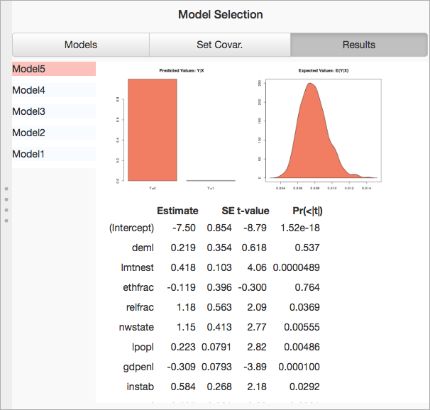
In the Results tab, all five models will be listed, as seen in figure 3. Click on the models to toggle through the results. For a complete replication script in R, including all system information necessary for a complete replication of your results, click on the Replication link in the lower left.

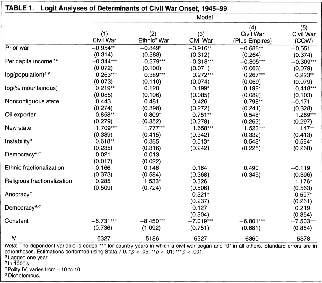
These results should be identical to the results in Fearon and Laitin’s Table 1, which appears below:

4 Extensions

At this point, it is straightforward to perform additional robustness checks or extensions on any of these five models using variables in the data.

For example, notice that there is a dummy variable in the data called colfra. This variable indicates whether the state is a former French colony. On a different sample, Collier and Hoeffler (2002) investigate whether being a former French colony makes one less likely to experience a civil war. They find that the coefficient is negative, but not statistically significant at 0.05.

Using the Fearon and Laitin data, we can test the hypothesis that being a former French colony makes one less likely to experience a civil war by including the colfra variable in Fearon and Laitin’s model.

• Replicate the construction of Model #1
• Add colfra as an independent variable
• Click Estimate

As we can see, the coefficient is negative, but not statistically significant at 0.05. This is consistent with the findings in Collier and Hoeffler (2002).

References